Elastic ViTs from Pretrained Models without Retraining

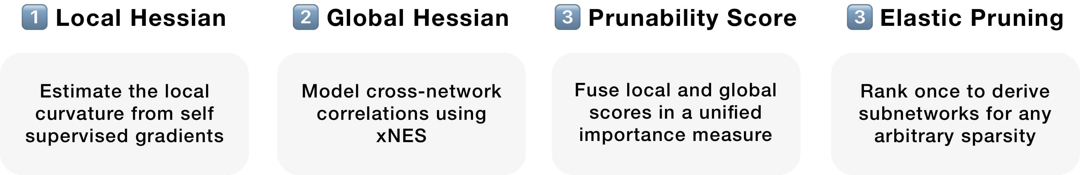
Figure 1: Overview of our method. We make pretrained models elastic in four steps: 1️⃣ we estimate the local inter-layer curvature via self-supervised gradients, 2️⃣ we model cross-network structure interactions via an evolutionary algorithm, 3️⃣ we fuse local and global scores in a unified importance measure, and 4️⃣ we rank structures once to derive subnetworks for any arbitrary sparsity.

This section briefly illustrates the key ideas behind our method. For more details, please refer to the paper.

The importance of a parameter can be expressed by the change it induces in the objective function \( \mathcal{L} \) when perturbed or removed. Following common practice, we approximate the loss variation under a small perturbation \( \delta\boldsymbol{\theta} \) as: \[ \begin{align} \delta \mathcal{L} &= \nabla_{\boldsymbol{\theta}}\mathcal{L}^{\top}\delta\boldsymbol{\theta} + \tfrac{1}{2}\delta\boldsymbol{\theta}^{\top}\mathbf{H}\delta\boldsymbol{\theta} + \mathcal{O}(\|\delta\boldsymbol{\theta}\|^3). 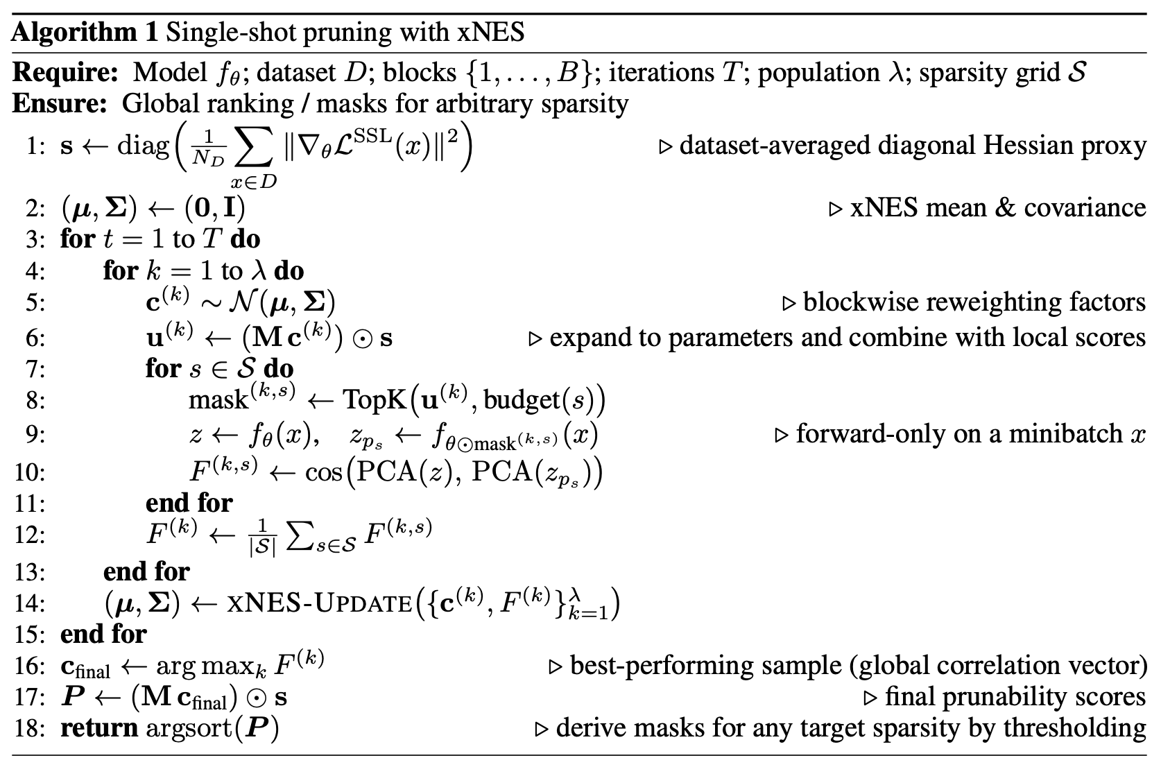\end{align} \] Assuming the model is near a local minima, the gradient term \( \nabla_{\boldsymbol{\theta}}\mathcal{L}^{\top}\delta\boldsymbol{\theta}\!\approx\!0 \) vanishes, and the Hessian \( H \) remains the dominant sensitivity indicator. Computing the whole Hessian is intractable as it scales quadratically with the number of parameters. Thus, we approximate it via a local term \( H^{(l)} \), i.e., the Hessian diagonal, capturing intra-block sensitivities and a global term \( H^{(g)} \), which models the off-diagonal interactions between functional structures such as transformer blocks and attention heads, via an evolutionary algorithm. We first 1️⃣ estimate the local curvature as: \[ \boldsymbol{H}^{(l)} \approx \frac{1}{N_D} \sum_{i=1}^{N_D} \left\| \nabla_{\boldsymbol{\theta}} \mathcal{L}_i \right\|^2. \] To obtain gradients in a model-agnostic way, we adopt the self-supervised DINO objective, removing the dependency on a classification head, and allowing the pruning of both supervised and self-supervised models. We then 2️⃣ estimate cross-network interactions via the Exponential Natural Evolution Strategy (xNES) by simulating pruning and measuring sensitivity directly. To do so, we sample individuals \( \mathbf{c}\!\sim\!\mathcal{N}(\boldsymbol{\mu},\boldsymbol{\Sigma}) \) which represent structure-wise reweightings. For each individual, we rescale the local sensitivity scores, compute pruning masks, prune and measure the divergence in cosine similarity between features from the original and pruned models. The genetic algorithm optimization evolves \( \Sigma \) towards the inverse of the true cross-structure Hessian. While this is an approximation, in practice the off-diagonal terms of \( \Sigma \) evolve to mirror cross-structure dependencies and form a tractable approximation of the global cross-structure Hessian. 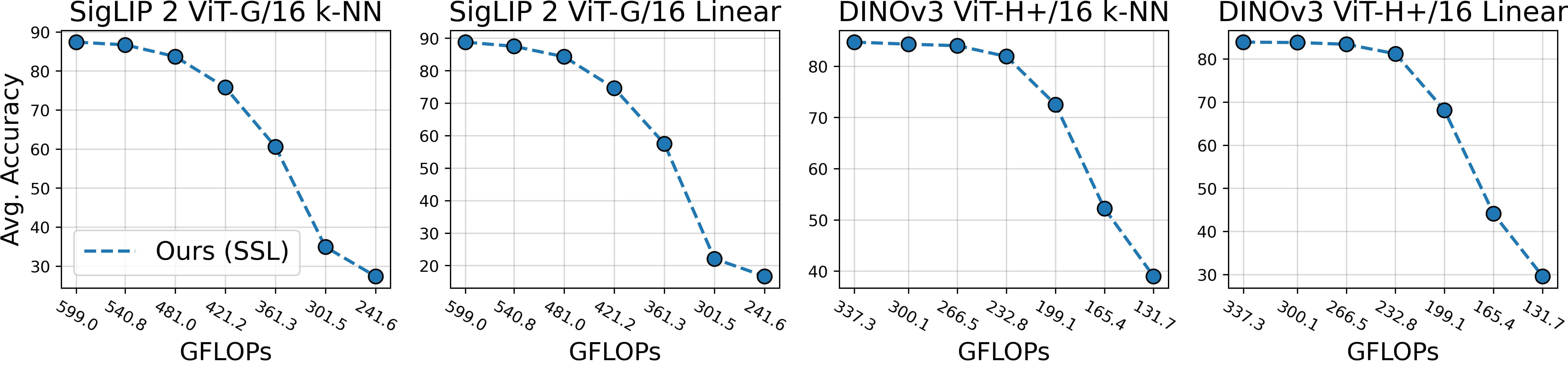We then 3️⃣ compute the prunability score for each parameter as \[ \begin{align} \boldsymbol{P} &= \operatorname{diag}\!\Bigg( \frac{1}{N_D}\sum_{i=1}^{N_D} \big\| \nabla_{\boldsymbol{\theta}}\, \mathcal{L}^{\mathrm{SSL}} \big\|^{2} \Bigg) \;\odot\; \mathbf{M}\,\boldsymbol{c}, \end{align} \] where \( M \) is a membership matrix \( \mathbf{M}\!\in\!\{0,1\}^{N\times B} \) that expands scaling factors \( c_i \) to all parameters within the corresponding structure. Scores are then aggregated on a per-structure basis by averaging. After computing \( \boldsymbol{P}\), we 4️⃣ globally rank all structures (or parameters) to determine the pruned subset at any desired sparsity level \( S \) \[ \Theta_S = \bigl\{ \theta_i \in \Theta \mid \operatorname{rank}(P_i) < |\Theta|\,(1-S) \bigr\}, \] where \(\Theta\) is the complete parameter set and \(P_i\) denotes the score of parameter \(\theta_i\). This global ranking enables single-shot pruning, as any target sparsity \( S\!\in\![0,1] \) can be realized without retraining, Hessian storage, or additional optimization.

We evaluate retraining-free models pruned to six evenly spaced sparsity levels from 10% to 60% on k-nearest neighbor and linear classification over seven datasets, and on linear semantic segmentation on Pascal VOC 2012. For classification experiments, we report the average top-1 accuracy averaged over seven datasets, and for semantic segmentation we report the mean Intersection over Union (mIoU). We compare our one-shot-all-sparsities approach to state-of-the-art pruning methods that produce one sparse model per run, or use multiple shots for each sparsity level. As other methods require a classification head, we use AugReg and DeIT ViT-B/16 backbones for a fair comparison.

The results, shown in Figure 2, demonstrate that our method matches or improves upon the state-of-the-art, especially at high sparsity ratios, by up to 7% and 12.3% in linear classification over SNIP Magnitude and FPTP, respectively, at 50% sparsity.

Figure 2: Our method matches or improves upon the state-of-the-art in a retraining-free setup, while not using labels. Top-1 accuracies in k-nearest neighbor and linear classification averaged across 7 datasets for supervised AugReg and DeIT ViT-B/16 models. Our label-free method outperforms or matches baselines that utilize labels, especially at high sparsity ratios.

The results for linear semantic segmentation are shown in Figure 3, and demonstrate that our method yields strong performance improvements at high sparsity ratios, improving by 9.1% over SNIP Magnitude at 50% sparsity for an AugReg ViT-B/16 backbone and by 15.3% over NViT at 60% sparsity for a DeIT ViT-B/16 backbone. Beyond linear segmentation, we use the in-context semantic segmentation framework from HummingBird to probe the quality of dense representations in DINOv1 ViT-B/16 models pruned using our method. We visualize the segmentation maps interactively across 50 pruning ratios for selected images below.

Figure 3: Our method retains segmentation performance best. mIoU on Pascal VOC 2012 for the linear semantic segmentation evaluation for AugReg and DeIT ViT-B/16 models.

We also use our method to prune self-supervised foundation models such as DINOv1, DINOv3, and SigLIPv2. The results, shown in Figures 3 and 4, show that our method yields strong sub-networks from DINOv1, pruning it to 40% sparsity with an accuracy drop of under 5% for both k-nearest neighbor and linear classification. On the contrary, we find that models that undergo large-scale pretraining (1.7B and 10B images respectively for SigLIPv2 and DINOv3) are harder to prune, benefit from longer optimization horizons (500 genetic algorithm iterations compared to a baseline of 50), and optimizing for more sparsities. Nonetheless, we improve over the second-best method in linear classification by up to 21.7% and 34.3% for SigLIPv2 and DINOv3, respectively.

Figure 4: Our method yields strong sparse sub-networks from DINOv1 ViT-B/16. Top-1 accuracy in k-nearest neighbor and linear classification averaged across 7 datasets for DINOv1 models pruned with our method, LAMP, and SNIP Magnitude.

Figure 5: Large-scale pretraining complicates pruning. Top-1 accuracy in k-nearest neighbor and linear classification for pruned DINOv3 and SigLIPv2 ViT-B/16 models. We find that self-supervised models trained on large datasets are harder to prune, benefit from longer optimization horizons, and optimizing for more sparsity.

While not a core component of our method, we also evaluate the performance of our pruned models after a single SparseGPT-style weight correction step or full fine-tuning. We benchmark our method plus post-pruning corrections against comparable state-of-the-art methods. The results, shown in Figure 6, show that our method either matches or improves upon the state-of-the-art, often by a large margin. In particular, we match and often improve over the LLM Surgeon, which performs five weight correction steps per sparsity level. Furthermore, a single weight correction step can largely restore the performance of SigLIPv2 ViT-B/16, yielding a 50% sparse model with a negligible accuracy drop in linear classification.

Figure 6: Weight correction helps retain post-pruning performance. A single weight correction step greatly improves performance at high sparsity levels while preserving efficiency. Our method matches or surpasses state-of-the-art baselines across pruning ratios (top row) and preserves self-supervised model accuracy even under extreme sparsity (bottom row).

We also compare our method to prior techniques that perform full-fine tuning post-pruning. For this, we use a DeIT ViT-B/16 backbone pruned to 50% sparsity with our method, and fine-tune it for 300 epochs on ImageNet-1k using the same protocol as NViT. In Table 1, we report the performance of our method on ImageNet and compare it against author-reported results. Furthermore, for open-weights models, we also evaluate the average performance across the seven benchmark datasets, and find that our method generalizes better, even while performing worse on ImageNet-1k compared to NViT.

Table 1: ImageNet-1k full fine-tuning recovers performance for 50% pruning. Our method fully recovers pre-pruning performance on ImageNet-1k and is competitive with other state-of-the-art approaches on ImageNet-1k, while generalizing better in k-nearest neighbor and linear classification.

We evaluate our method on the entire DeiT-III family, from a ViT-S/16 to a ViT-H/14, and we find that larger models can be pruned more aggressively with a minimal loss in performance. For example, pruning a ViT-H/14 to 50% sparsity, equivalent to removing 316M parameters, only results in a 3.7% and 3.4% average accuracy drop in k-nearest neighbor and linear classification, respectively. When post-pruning weight correction is applied, performance is mostly restored, with an average drop of 0.5% and an improvement of 0.9% in k-nearest neighbor and linear classification, respectively. Interestingly, weight correction does not improve performance for the ViT-S/16 model at 50% sparsity and further. We hypothesize this might be due to the limited remaining representational capacity, as a 50% sparse model has only ~11M parameters left.

We also attempt to prune huge self-supervised models: a SigLIPv2 ViT-G/16 and a DINOv3 ViT-H+/16. Figure 8 shows that they both retain performance up to 30% sparsity, with accuracy dropping sharply beyond that, in contrast with our findings for DeIT-III ViT-H/14. We hypothesize this might be due to large-scale pre-training, as DeIT-III is trained on ~13M images, while SigLIPv2 and DINOv3 are trained on 1.7B and 10B images, respectively. Large-scale pre-training likely distributes knowledge more evenly across the model, making it harder to prune. Nonetheless, weight correction can recover performance for models that underwent large-scale pre-training, as shown in Figure 6 for SigLIPv2 ViT-B/16.

Figure 7: Pruning the DeIT-III family. Top-1 accuracy in k-nearest neighbor and linear classification averaged across 7 datasets for DeIT-III models from S/16 to H/14 pruned with our method, with and without weight correction.

Figure 8: Huge models are not necessarily more prunable. Top-1 accuracy in k-nearest neighbor and linear classification averaged across 7 datasets for DINOv3 ViT-H+/16 and SigLIPv2 ViT-G/16 models pruned with our method. Contrary to a DeIT-III ViT-H/14 backbone, performance quickly degrades beyond 30% sparsity.